We present an efficient algorithm for preserving
the total volume of free-form solids undergoing deformation using discrete
level-of-detail representations. Given the boundary representation of a
solid and user-specified deformation, the algorithm utilizes augmented
Lagrangian methods to compute the new node positions of the deformation
lattice, while minimizing the elastic energy subject to the volume-preserving
criterion. During each iteration, the non-linear optimizer computes the
volume deviation and its derivatives based on a triangular approximation
method, which requires a finely tessellated mesh to achieve desirable accuracy.
To reduce the computational cost, we exploit the multi-level representations
of the boundary surfaces to greatly accelerate the performance of the non-linear
optimizer. This technique also provides interactive response to the users.
Furthermore, it is generally applicable to lattice-based free-form deformation
and its variants. Our implementation has been applied to several complex
solids. We have been able to achieve an order of magnitude performance
improvement over the traditional methods on our test models.
Motivation
Engineering design and shape styling often require the capability to manipulate flexible objects, including bending, twisting, compressing or stretching parts of the model or its entire geometry. Several modeling techniques and design methodologies have been proposed to provide intuitive manipulation and interactive deformation of flexible objects. One of the most versatile and powerful tools for representing and modeling flexible objects is free-form deformation (FFD) or space deformation introduced by Sederberg and Parry. FFD unifies both the free-form surfaces and solid modeling into a common framework for deforming solid geometry in a free-form manner. Furthermore, it can also sculpt surfaces and polygonal models. A more general extension to FFD (EFFD) was later presented by Coquillart.
However, none of these methods associates any physical constraints with geometric deformation of solids. Recently, the integration of geometric design and physically-based modeling techniques has emerged to be an attractive alternative, as a natural and systematic approach to constraint-based design, shape blending and a variety of solid modeling problems by several researchers. Principles of physics govern the dynamic behaviors of objects in the physical world. Direct manipulation and interactive sculpturing of geometric models should also be compliant with the law of physics to give designers and stylists an intuitive grasp of the object. One of the important governing laws of Newtonian physics is the conservation of mass. When the density of a given material is constant, this implies the preservation of volume.
A volume-preservation constraint allows designers
to keep the required relative proportionality of object sizes (in terms
of their volumes) in the design of a complex assembly consisting of multiple
parts. Another example is the design of a container whose capacity is given
a priori. The volume inside should be preserved when the designer modifies
the shape of the container. Volume-preserving free-form deformation is
not only a useful tool for modeling, but can also be a powerful visual
aid in engineering animation and virtual prototyping as well. This technique
can also be used to automatically create the standard squash and stretch
effects in computer animation and help bring life to the animated characters.
Main Contribution
We present a new approach for volume-preserving free-form deformation using multi-level-of-detail representations. Our method is
Although our implementation is based on the trivariate
Bernstein basis FFD, the proposed technique is generally applicable to
other lattice-based free-form deformations and their variants. Our implementation
allows the designer to interactively manipulate the free-form solids and
to view the model changes due to deformation in real-time, while simulating
the physical behaviors of the solids subject to the volume-preserving constraint.
We have been able to achieve an order of magnitude speedup over the conventional
optimization methods.
Implementation & Results
We have implemented our algorithm in C++. The image generation and the user interface are developed using the OpenGL and GLUT library. All timing data were obtained on an SGI Onyx2 with 195MHz R10000 MIPS processors.
We have tested our system on various models undergoing deformation. The color images are also available at our web site (http://gamma.cs.unc.edu/ffd). We analyze its performance using four examples here.
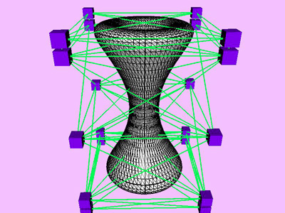
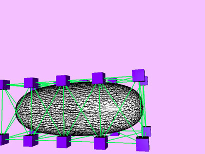
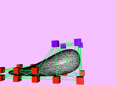
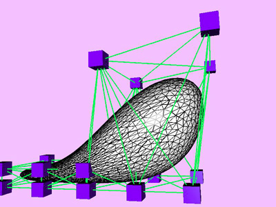
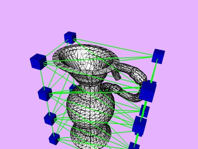
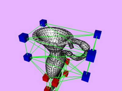
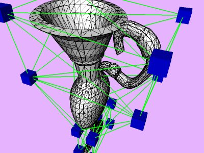
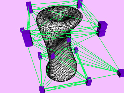
Table 1 shows the performance improvement of the multi-level optimization over the usual optimization method. We have consistently achieved about an order of magnitude speedup using the multi-level optimization. The torus stretch example has an interesting property that is worth mentioning. If we start the algorithm from a fine mesh (NTri³ 4096), the shape converges to a different configuration than if we start with a coarse mesh (Plate 6). This is not surprising because there are often multiple local minimum states in many near symmetric constraints. Our method seeks only the local minimum, therefore the result may not be consistent for different starting levels. Plate 7 is an example of very large deformation. The rounded club is bent significantly. Our algorithm handles these situations without any numerical problem. In Plate 5, The bottom half of a water pitcher model (6176 triangles) is compressed by the user. As a result of optimization, the upper part is expanded.
Figure 5: Convergence Curve. Torus compression.
Figure 6: Convergence Curve. Stretched Torus.
Figure 7: Convergence Curve. Rounded Club Partial Compression.
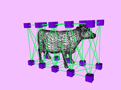
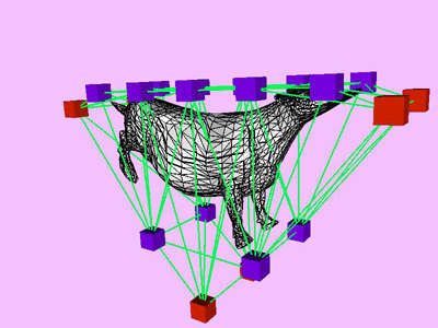
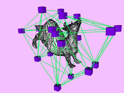
Figure 8: Convergence Curve. Bending Cow.
Table 1: Performance Improvement by Multi Level
Optimization. T1 and T2 are the total
CPU time (msec) of without and with Multi Level Optimization respectively.
D V/Vorg
is the final relative volume deviation after Multi-Level Optimization.
NTri is the number at the terminal level.
| Example |
|
|
|
|
|
| Torus
Compression |
21000
|
1760
|
12
|
4096
|
0.05%
|
| Torus Stretch |
677400
|
11080
|
61
|
65536
|
0.08%
|
| Club Partial
Compressioin |
40990
|
3530
|
12
|
16384
|
0.07%
|
| Cow Bending |
15810
|
2240
|
7
|
5804
|
0.07%
|
 |
 |
 |
 |
 |
 |
 |
 |
 |
 |
 |
 |
 |
 |
 |
 |
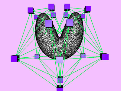 |
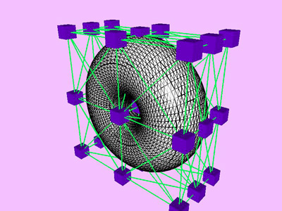
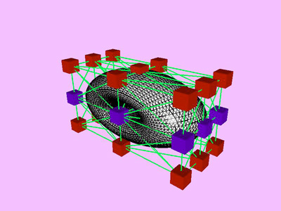
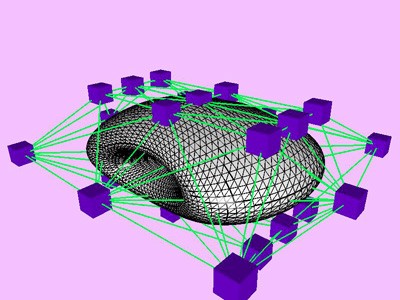
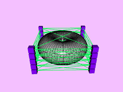
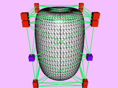
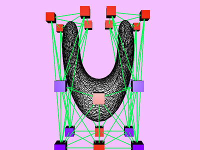
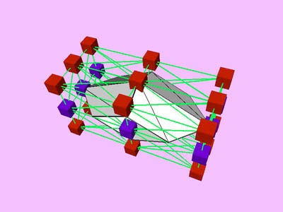
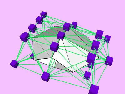
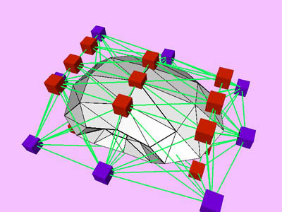
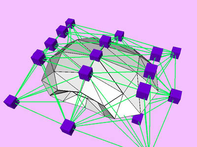
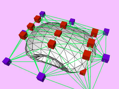
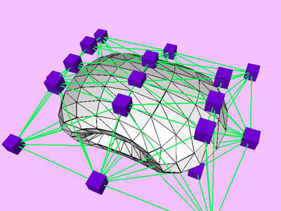
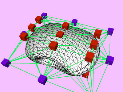
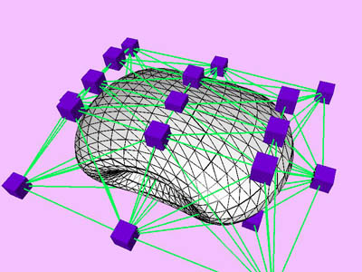
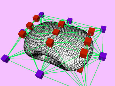
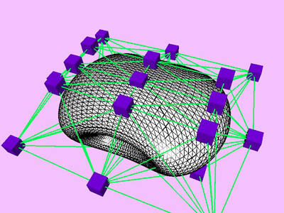
Table
2: Performance chart of multi-level optimization for a compressed torus
example (Plate 1). The level k corresponds to the minimization at
the kth level of approximation with NTti
triangles. Red and blue cubes denote fixed and free nodes respectively.
Node points X(k), penalty factor s
(k), and Lagrange multiplier l
(k) are inherited from one level to the next. D
X is the maximum change in the coordinates of node points X
relative to the size (the maximum extent) of the object. Nstep
is the total number of internal minimization steps at each level.
T is CPU time (in msec) spent for the minimization of the kth
level. Tc is cumulative CPU time.
|
|
|
|
|
|
|
|
|
|
|
|
 |
 |
|
|
|
|
|
|
|
 |
 |
|
|
|
|
|
|
|
 |
 |
|
|
|
|
|
|
|
 |
 |
|
|
|
|
|
|
|
 |
 |
|
|
|
|
Copyright 1998. Permission to reprint/republish this material for advertising or promotional purposes or for creating new collective works for resale or redistribution to servers or lists, or to reuse any copyrighted component of this work in other works must be obtained from the authors.
This material is presented to ensure timely dissemination of scholarly and technical work. Copyright and all rights therein are retained by authors or by other copyright holders. All persons copying this information are expected to adhere to the terms and constraints invoked by each author's copyright. In all cases, these works may not be reposted without the explicit permission of the copyright holder.