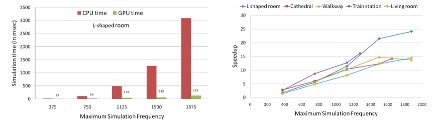
| We investigate the performance of ARD solver on varying maximum usable simulation frequency v_max. (Left) Simulation time (in ms) per time-step of CPU-based and GPU-based adaptive rectangular decomposition (ARD) solver with varying v_max for the L-shaped room scene. Note that the GPU-based solver is 24 times faster at highest v_max. (Right) Speedup (=CPU time/GPU time) achieved by our GPU-based ARD solver over the CPU-based solver with varying v_max for the different test scenes. For v_max > 1300 Hz, we achieve a speedup of 10-25X.
|
|
|
| |
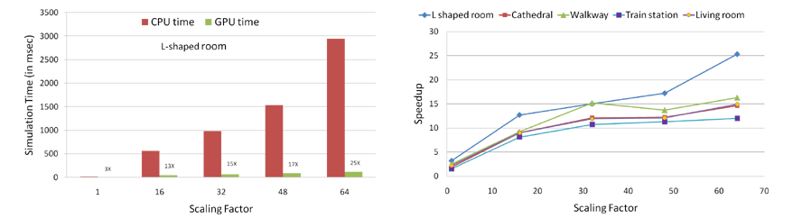
| We investigate the performance of ARD solver on varying scene volume. For both figures, we scale the original volume of the test scenes by the Scaling Factor. Maximum usable simulation frequency v_max values used are : L-shaped room(450Hz), Cathedral(412Hz), Walkway(472Hz), Train station(285Hz) and Living room(487Hz). (Left) Simulation time (in msec) per time-step of CPU-based and GPU-based adaptive rectangular decomposition (ARD) solver with varying scene volume for L-shaped room scene with v_max = 450 Hz. Note that the GPU-based solver is 25 times faster at highest scaling factor. (Right) Speedup (=CPU time/GPU time) achieved by our GPU-based ARD solver over the CPU implementation with varying scene volume for the different test scenes. As the scene volume increases, we achieve a higher speedup. For 64 times the original volume, the speedup becomes 12-25X.
|
|
|
| |
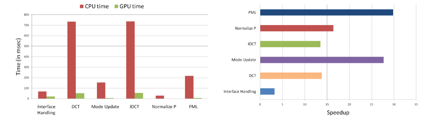
| For the walkway scene of air volume 6411 cubic meters at maximum usable simulation frequency v_max of 1875 Hz : (Left) Simulation stages - Interface handling, discrete cosine transform (DCT), mode update, inverse discrete cosine transform (IDCT), normalize pressure and perfectly matched layer (PML), and the corresponding time spent in the CPU-based and GPU-based adaptive rectangular decomposition (ARD) solver. For our GPU-based solver, almost all the stages of the simulation stage are more or less balanced, except mode update and normalize pressure, whose costs become negligible. (Right) Speedups achieved by individual stages of the GPU-based ARD over the CPU-based solver - PML(30X), mode update(28X), normalize pressure(16X), DCT(14X), IDCT(14X) and interface handling(3X). Due to uncoalesced memory access nature of interface handling, speedup obtained is nominal. But since its contribution to the total running time is far less compared to other steps, it does not become a bottleneck.
|
|
|
| |
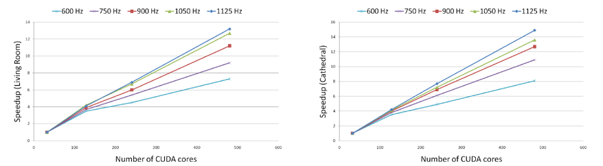
| We use Cathedral and living room as our benchmark and run the simulations with varying maximum usable simulation frequency v_max on 4 different NVIDIA GPU's with different number of CUDA processors( also called cores) - GeForce 9600M GT (32 cores), GeForce 8800GTX (128 cores), Quadro FX 5800 (240 cores) and Geforce GTX 480 (480 cores). We calculate the speedup with respect to the GPU with least number of CUDA cores (32 cores) i.e. Speedup on GPU with X cores = (Simulation time on 32-cores GPU)/(Simulation time on X-cores GPU). We achieve linear scaling in performance at higher values of v_max. As the number of cores increase from 32 to 128 (4 times), our GPU-based adaptive rectangular decomposition (ARD) solver becomes 4X faster. Similarly from 32 to 240 cores(7.5 times increase), we get 7-7.5X speedup and for 32 cores to 480 cores (15 times), we are 14-15X faster.
|
|
|
| |
| We plot speedup achieved by CPU-based and our GPU-based adaptive rectangular decomposition (ARD) solver over CPU-based finite-difference time-domain (FDTD) solver with varying maximum usable simulation frequency v_max for the small room benchmark scene. Our CPU-based FDTD solver is based upon the work proposed by Sakamoto et al. We calculate the speedup of both the ARD solvers over FDTD as (simulation time per time-step for FDTD)/(simulation time per time-step for ARD). FDTD runs out of memory from v_max > 3750 Hz for this scene. We use projected time to calculate FDTD timings above 3750 Hz. The CPU-based ARD solver achieves achieves a maximum speedup of 75X over CPU-based FDTD. On the other hand, our GPU-based ARD solver achieves a maximum speedup of 1100X over CPU-based FDTD.
|
|
|
| |