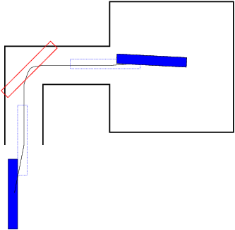
Given an environment, computing a collision free trajectory for a rigid body from an initial configuration to a goal configuration is a classic problem in robotics literature. This problem has been extensively studied and a number of algorithms have been proposed [Lat91]. Recently Latombe classified earlier approaches to motion planning into two categories:
Main Contribution: We present a hybrid path planning algorithm for free-flying, rigid bodies translating and rotating in a 3D workspace. Our approach utilizes global geometric analysis of the workspace to generate an approximate path in configuration space. We then identify invalid segments of this estimated path, for which the configurations in the estimated path cause the robot to collide with the obstacles. We complete the query by computing linking subpaths or ``bridges'' [CL93]to replace the invalid segments. These bridges are generated by a randomized planner with carefully restricted sampling around narrow passages.
Our geometric analysis uses a discrete approximation of the generalized Voronoi diagram (GVD) of the workspace, computed using graphics hardware [HCK+99]. Unlike classical criticality based methods, the approximate GVD computation is fast and simple to implement. It gives us information about the configuration space that is global in nature, but not necessarily complete.
The two key distinctive features of our approach are:
The rest of the paper is organized as follows. In Section 2 we discuss related work. In Section 3 we introduce terminology related to the Voronoi diagram, and in Section 4 we explain our algorithm. In Section 5 we give implementation details and present performance results. In Section 6 we analyze the performance of the algorithm, and in the final section we conclude and indicate areas of future work.
In this section we survey earlier related work.
Generalized Voronoi diagrams have long been used as a basis for motion planning algorithms [ÓSY83,CB95,CB96,WAS99a]. The GVD represents the connectivity of a space but has a dimension lower by one, and (in three dimensions) it is composed of surfaces of maximal clearance.
The disadvantage of using the GVD has always been that it is difficult to compute robustly and efficiently. Recently, several approaches to this problem have been proposed. Vleugels and Overmars [VO95]give an algorithm that applies spatial subdivision and isosurface extraction techniques to acquire an approximate model of the diagram. More recently, Wilmarth, Amato, and Stiller [WAS99a,WAS99b]have shown how points on the GVD can be found without computing a representation of the entire set. Finally, Hoff et al. [HCK+99]have introduced a method that uses graphics hardware to generate a discrete model at a specified resolution. We use this latter method in our work.
The Voronoi diagram can be used in several ways:
Recently a class of randomized algorithms known as Probabilistic Roadmap Methods (PRMs) have been shown to be very successful for many planning scenarios [KL94,HLM99]. The original PRM planner [KL94]generated samples at random in configuration space, attempting to connect each sample by a simple C-space path to one of the points already found. Over time, the graph thus produced will tend to represent the connectivity of the C-space reasonably well, and a query can be rapidly performed by linking the search points to the graph and then searching the graph. Many variations on this idea have been developed. The planner we use as a baseline for performance comparison and as a subroutine in our work is described in [HLM99]. Some details of its algorithm are given in Section 4.4.
Generalized Voronoi Diagram: Let a set of geometric objects, or sites, be denoted s1, s2,..., sn. For each site si, define a distance function di(x) = dist(si,x). The Voronoi region of si is the set Vi = {x | di(x) � dj(x) "j � i}.
The collection of regions V1, ..., Vn is called the generalized Voronoi diagram or GVD, which partitions the space into cells suitable for proximity queries.
The (ordinary) Voronoi diagram corresponds to the case when each si is an individual point. The boundaries of the regions Vi are called Voronoi boundaries, which are loci of points equidistant to at least two sites. Sometimes we use the term GVD to refer to the union of the Voronoi boundaries, rather than the collection of Voronoi cells. In three dimensions, the intersection of two Voronoi regions is a Voronoi face, the intersection of at least two Voronoi faces is a Voronoi edge, and the intersection of at least two Voronoi edges is a Voronoi vertex. Together the Voronoi edges and vertices form a graph, the generalized Voronoi graph (GVG). For sites such as points, lines, polygons, and splines, the Voronoi diagram is composed of portions of algebraic curves and surfaces.
Our hybrid planning algorithm can be outlined as follows.

Our method for computing the generalized Voronoi diagram is based on the algorithm presented by by Hoff et al. [HCK+99]. It relies on the ready availability of standard Z-buffered graphics hardware. The color buffer stores the attributes (intensity or shade) of each pixel in the image space; the depth buffer (Z-buffer) stores the depth of every visible pixel. Given the vertices of a triangle, the rasterization hardware interpolates depth linearly across the triangle's interior. All raster samples covered by a triangle have an interpolated depth.
We compute a discrete Voronoi diagram by rendering a three-dimensional distance mesh for each site. The 3D polygonal distance mesh is an approximation of a possibly non-linear distance function over a plane. Each site is assigned a unique identifying color, and the corresponding distance mesh is rendered in that color using a parallel projection. The graphics system performs a depth test for each pixel in order to resolve the visibility of surfaces. The depth buffer maintains the minimum depth at each point as polygons are rendered. When the minimum depth is updated, the frame buffer is also updated with the pixel's color. Thus, the rasterization provides, for each pixel, the identity of the nearest site (encoded as a color) and the distance to that site (encoded as a depth value).
For the 3D workspace, we generate the Voronoi diagram in slices. For each slice and each Voronoi site, there is a distance function giving the distances in R3 from points on the slice to the given site. The graphics system renders and composites these distance functions as described above to produce a single slice of the discrete Voronoi diagram.
We compute the generalized Voronoi graph by scanning the resulting pixel map, two slices at a time, seeking locations whose neighboring pixels exhibit at least three different colors. We store the resulting locations in an edge list representation. The vertex data structure contains the coordinates of the point and the clearance distance to the obstacles (because it is a Voronoi vertex, the point will be equidistant to at least four sites). The edge data structure has a list of sampled coordinates of points on the edge, and the minimum clearance distance for the whole edge. Note that all the sample points are restricted to a uniform grid, so that the vertex and edge points do not lie on the actual Voronoi boundaries, but instead on nearby grid points.
After generating the GVG, we use it to find an approximate path in the workspace for the robot to follow, called the workspace path. Define a query configuration to be an initial or goal configuration, and a query location to be the projection to R3 of a query configuration. Then the workspace path links the initial and goal query locations.
Before we can search the GVG for a path, we need to link the query locations to the GVG. To link a query location, we first determine the Voronoi cell containing it. We then compute line segments from the query location to each Voronoi vertex of the cell, and eliminate any segments that pass through obstacles.
We add the query locations and their linking line segments to the GVG data structure as (formal) Voronoi vertices and edges. Each newly added edge contains a list of points and the value of the minimum distance to the environment.
After linking the query locations to the GVG, we use a generalized single-source shortest paths algorithm, where the length of a path is determined by a combination of the Manhattan distance along the path and the maximal clearance over the whole path. This path, the workspace path, is a solution to the query for a point robot, and it satisfies a partial criterion of maximal clearance.
After finding the workspace path, we must choose an orientation for the robot at each point on the path. To do this, we determine a major axis for the robot, and align it with the tangent vector of the path, as determined by a finite difference estimate.
For a complex shape, there are many reasonable definitions of the ``major axis.'' For our purposes, we want an axis around which the robot fits as tightly as possible. To determine such an axis, we use linear regression to compute a best-fit line approximating the vertices of the robot. This line is chosen to minimize the root mean square of the (Euclidean) distances of the vertices to the line. The origin of the robot is defined to be the center of gravity of the vertices.
Once we have determined how to align the specified major axis of the robot, it is still free to rotate about that axis. The choice of orientation about the major axis (i.e., the ``roll'') on any geometric information is made arbitrarily. We simply make sure that, up to discrete approximation, the orientation varies continuously as the robot traverses the path.
In this section, we explain how the estimated path is modified into a final path for the robot. First, using a simple straight-line local planner, we attempt to connect each configuration with its successor. Configurations for which the robot is colliding with the obstacles, or which cannot be connected to a neighbor, are marked ``invalid''.
The path has now been decomposed into valid segments, for which the robot is free, alternating with invalid segments, for which it is not. For each invalid segment, we apply the randomized planner [HLM99], with initial and goal configurations biased by the tangent vectors of the GVG. This planner maintains trees of free configurations rooted at the start and finish. At each iteration (called an expansion iteration), it chooses a configuration p from one of the trees, generates new configurations in a neighborhood of p, and retains those which can be linked to p by a free path. The local planner terminates when the two trees are connected. This algorithm automatically biases sampling towards configurations known to be free.
The query configurations for the randomized planner are the valid configurations immediately preceding and following the invalid segment. The configuration space for the planner is defined to be the tightest axis-aligned box that contains bounding balls for the robot at both query locations. See Figure 2.
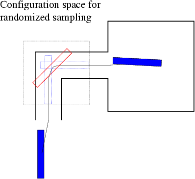
It is possible for the robot to get into a tight spot for which the restricted configuration space does not provide enough room for the robot to maneuver from the beginning of the invalid segment to the end of it. To handle such situations we use a simple expedient: If, after a fixed number of expansion iterations, the planner has not linked the two ends of the invalid segment, the planner's configuration space is enlarged to the full original C-space, and randomized planning is resumed. If this is not successful after another predetermined number of iterations, then it is assumed that the heuristics guiding the initial path estimate have failed, and the planner simply uses other planning methods (i.e., PRM in our current implementation) to link the original start to the original finish.
While an invalid segment is being bridged, what was a narrow passage on the scale of the entire scene is now a relatively open area within the restricted configuration space (see Figure 2). However, there may be a portion of the invalid segment which constitutes a narrow passage even on this smaller scale. To increase sampling in these bottleneck areas, we generate a new configuration near the narrowest point on the invalid segment (``narrowest'' being measured in terms of distance from Voronoi sites, i.e., the obstacles). We find the new configuration by uniform random sampling in a neighborhood of the narrowest point.
We then perform two randomized sampling steps, one linking the beginning of the invalid segment to the new configuration near the narrowest point, and the other linking the new configuration to the end of the invalid segment. The new configuration acts as a seed, causing a number of configurations to be generated near the narrowest point on the narrow passage.
If the Voronoi site distance at the narrowest point is greater than half the radius of the robot's bounding ball, then this operation is not performed since in practice we have found that a single randomized planning step works well in such cases.
We used several benchmark scenarios, described below:
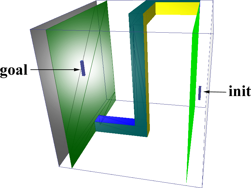
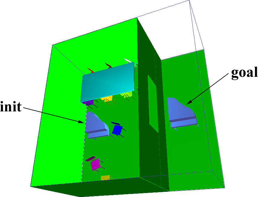
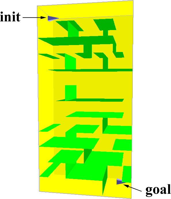
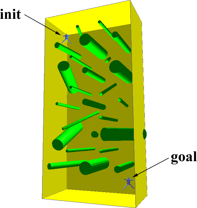
The results of the benchmarks are summarized in Table 5. Res gives the resolution, along the largest axis of the scene, at which the Voronoi graph was computed. GVG is the time for computing the Voronoi graph, Query the time for the query phase after the Voronoi graph was constructed, and PRM is the time for the randomized planner alone. Gain indicates the speedup factor using our hybrid planner (including preprocessing and query time) vs. the randomized planner with uniform sampling. All times are in seconds on a 300 MHz MIPS R12000 processor.
The randomized planner has several adjustable parameters that can affect performance. The timings for the randomized planner alone, as well as our new planner, reflect our best efforts to choose parameters that will give optimal performance for the given scene.
| Scene | Res | GVG | Query | PRM | Gain |
| 1 | 128 | 10.4 | 0.70 | 894 | 88 |
| 2 | 64 | 5.05 | 41.9 | 603 | 14 |
| 3 | 128 | 2.14 | 5.74 | 341.1 | 43 |
| 4 | 128 | 24.9 | 23.8 | 450 | 9 |
| 5 | 64 | 2.87 | 19.7 | 97.40 | 4 |
In this section, we discuss the performance of our planner. We consider properties of the robot and workspace that affect the performance, and we describe the approach of our planner to the problem of narrow passages.
We can make the following observations about the performance of our planner.
The planner also works well when the robot is organized compactly around a linear axis. In such cases, aligning that axis along the tangent of the Voronoi graph is likely to result in a free configuration.
Conversely, our use of the GVG provides relatively little benefit if the robot is large compared to the scene and has a highly complex shape.
In some cases, our simple analysis of the Voronoi graph may produce an estimated path that is not usable. If this happens, then the randomized planner will ultimately be called on the original query. We can set the number of randomized planning iterations that will be expended trying to bridge an invalid segment before the estimated path is abandoned. We generally choose the number of iterations on the assumption that the Voronoi based planner should succeed in a few tens of seconds. If it does not, then the scene is likely to be a difficult one for the randomized planner as well, so the time spent unsuccessfully trying to use the Voronoi diagram will be only a very small portion of the total planning time.
Here we consider in general terms the issue of narrow passages as it relates to our planner.
If there is a path for the robot which is, to the precision of our Voronoi computation, wider than the bounding ball for the robot, then our planner will generally find it very rapidly, with no resort to randomized planning. Thus, in the context of our planner, any region of the workspace wider than the bounding ball of the robot does not correspond to a narrow passage in C-space. We therefore define a workspace narrow passage to be a portion of the GVG for which the site distance is less than the radius of the robot's bounding ball. By the above observations, any C-space narrow passage corresponds to some part of a workspace narrow passage.
Because invalid segments are determined by collision of the robot with the environment, they can only occur in workspace narrow passages, or along a segment joining a query configuration to the GVG. Thus we see that our planner primarily uses randomized planning in a subset of the workspace narrow passages. It may seem paradoxical that narrow passages, which are notoriously difficult for randomized planners, are precisely where we use randomized planning. This strategy in fact works well because of the three techniques we use to bias sampling:
We initially restrict randomized planning to a region delimited by the endpoints of the invalid segment, increasing the chances that a sample will land in the narrow passage. Essentially, in the context of this restricted C-space, the narrow passage becomes a relatively open area.
When a passage is especially narrow, measured in terms of the workspace, we seed the PRM planner with an additional configuration near the narrowest point. These additional seed configurations have the effect of intensifying sampling in the most restricted areas.
We use a PRM planner that generates new samples near samples already found, and we initialize that planner with configurations (generated by the tangent vectors of the GVG) at both ends of the narrow passage. Because the PRM planner grows trees of configurations rooted at the two ends of the narrow passage, the trees have a high probability of growing into the narrow passage. This phenomenon is discussed in terms of expansive components in [HLM99]. Indeed, the chief benefit of the restricted C-space is to prevent the trees of configurations from immediately growing away from the narrow passage.
We have introduced a planner that uses simplified global geometric analysis to generate an estimated path, and then uses randomized planning guided by the generalized Voronoi diagram, to modify the estimated path into a collision free path. We have tested the planner on several benchmarks and found that it can be over an order of magnitude faster than a comparable purely randomized planner.
There are several possible directions for future research in extending this work.
We would like to thank Kenny Hoff for providing us his Voronoi computation software. We are also grateful to David Hsu and Jean-Claude Latombe for helpful discussion on PRM and providing us with an earlier version of their randomized planner. Finally, credits are due to Jean-Paul Laumond and Nicola Simeon for the dataset on the piano scene.
1Supported in part by ARO Contract
DAAH04-96-1-0257 and DAAG55-98-1-0322, NSF Career Award CCR-9625217,
NSF grants DMI-9900157 and NSF IIS-9821067, ONR Young Investigator
Award, and Intel.