• Final Objectives:
• Integrate Rigid Body Simulation with Collision Detection
• Determine and Implement a Rigid Body Sampling Solution
• Analyze Performance of the System
• Provide Topics for Further Research
• Implementation:
• The code:  The Demo Source

1. Rigid Body Implementation
• Class Code
2. Collision Detection
• Color and Depth Buffer
• Storing Contacts
3. Sampling a Rigid Body
• Dense vs. Sparse Sampling
• Boundary vs. Volume Sampling
• Penetration Depth
• Hardware Accelerated Sampling
4. Collision Rebound
• Impulse Based
• Physics Based
• Sampling the Depth Buffer for the Normal
• Alternative Normal Computation
5. ODE Solver
6. Performance Hints
7. Future Research
8. Conclusions

 
Rigid Body Implementation

class RigidBody
{
    Body      CenterMass;   // CENTER OF MASS
    Particles Samples;      // SAMPLING PARTICLES
}
class Body
{
    float  mass;            // MASS OF RIGID BODY
    float  position[2];     // x,y POSITION
    float  velocity[2];     // x,y LINEAR VELOCITY
    float  rotation;        // ROTATION IN DEGREES (z-axis)
    float  omega;           // ANGULAR VELOCITY (z-axis)
    float  force[2];        // x,y LINEAR FORCE
    float  torque;          // ANGULAR FORCE (z-axis)
}
typedef struct _Particle {
    float x,y;              // x,y POSITION RELATIVE TO CENTER MASS
} Particle;

class Particles
{
    int       NumParticles; // NUMBER OF PARTICLES
    Particle *P;            // ARRAY OF PARTICLES
}

    Looking at the various classes notice how the positions and velocities are stored for the x and y coordinates only.  Angular velocity (omega) and torque are implicitly defined for the z-axis, which is the axis of rotation in 2D.  In the previous system, I was storing vector and matrices, which are much larger and require more bookkeeping, which can be eliminated because there is no linear motion in the z-direction, and no rotation about the x-axis or y-axis.
    Using this streamlined version we can perform some tricks to speed up the simulation at the cost of some accuracy.  The description of how to compute rebound forces will be shown in detail later.

Collision Detection

Color and Depth Buffer

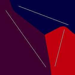
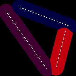
    The basic principle behind using the voronoi diagram for collision detection is to use a two pass algorithm.  The first pass through the system will draw the voronoi sites, into the back buffer.  Each site has a distinct color which is used as its id.  The geometry behind the voronoi diagram will not be discussed here.  Each pixel has a distinct color and depth.  The depth value is the distance to the voronoi site whose id is the color at the pixel.  A rigid body is theoretically composed of particles.  A particle in the system exists at a single pixel, by reading back the depth buffer it can determine if it is colliding with an object.  If the distance is within a certain distance tolerance then there is a collision between the particle and the voronoi site.  By reading the color buffer at the pixel location, the particle then knows which voronoi site it is in contact with.  How to correctly sample a rigid body into particles will be discussed in the next section.  Images below show the voronoi sites and associated depth buffer.

(click to enlarge)

Color Buffer

Depth Buffer

    The image on the left shows three voronoi line sites (click on picture for full size).  If we think of the voronoi diagram as a force field that is stronger the closer a particle is to the actual site, the path of least resistance is along the voronoi boundaries.  This is easily visible in the depth buffer image, where darker values are farther away from the voronoi sites.

Storing Contacts

    When a collision is detected, we must break from the ordinary ordinary differential equation solver and compute the updates.  To do this we store the contacts in a class.

typedef struct _ContactPoint {
  RigidBody *rb;               // BODY CONTAINING VERTEX
  int        siteID;           // VORONOI SITE ID
  float      pos[2];           // WORLD-SPACE VERTEX LOCATION
  float      n[2];             // OUTWARDS POINTING NORMAL OF VORONOI SITE
} ContactPoint;

class Contact
{
public:
  int NumContacts;
  ContactPoint *C;
}

    This class will allow for multiple contacts per timestep, which is useful if the solver can handle them.  What should normally happen is that the solver will backup to the instant of the first contact and solve the appropriate forces.  In rigid body simulation only one contact can happen at a single timestep.

    After the voronoi diagram has been read and collisions detected, the scene can then be drawn over the top of the voronoi diagram.  We only need to have the voronoi diagram for collision detection, it does not need to be present for the actual drawing environment.  Rigid body's may have a geometric representation with texture mapping, as well as the voronoi sites.  This shows the advantages multipass rendering and how the graphics hardware can be used for many ways.

Sampling a Rigid Body

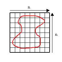
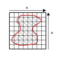
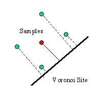
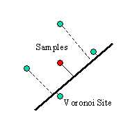
Sparse Boundary Sampling

Dense Boundary Sampling

    The answer is: "It depends on the situation!"  What if there is a simulation with many bodies, and some bodies require very accurate collision detection, and others do not, then a different sampling density for both bodies is needed.  What we want to do is allow the user to specify the sampling density for each rigid body at the start of the simulation.  This can be accomplished in various ways.  A simple way to do this is to have the user supply the sampling points in a datafile.  Below is a sample datafile for a square with 3 samples per edge, no samples in the interior (8 samples).

8                        // NUMBER OF SAMPLES
10    0 0   0 0  0  20   // CENTER MASS - MASS, X,Y, VX, VY, ROTATION, OMEGA
-0.3 -0.3
 0.0 -0.3
 0.3 -0.3
 0.3  0.0
 0.3  0.3
 0.0  0.3
-0.3  0.3
-0.3  0.0

    This allows the user to have to complete control over the sampling density.  This solution allows for specification of non-uniform sampling of arbitrary shaped objects, since the sampling is what essentially defines the boundary of the object.

Boundary vs. Volume Sampling

    Two different styles for sampling can be used, each providing their own set of benefits.  When simulating we can specify the timestep to be any value, therefore making it small enough to detect surface collision.  If this is the case, then we need to only sample the boundary of the rigid body.  Since we are detecting contact at the surface, any point inside the boundary will never be used, which is still being tested.  Eliminating the inner sampling points will dramatically reduce the computation per timestep since only the boundary is being tested.  For example, if we have a square rigid body with n samples per edge, we only have to test 4n samples per timestep.  If we sampled the entire volume we would have n² tests per timestep.  An order of magnitude savings in sampling only the boundary.

Boundary Sampling

Volume Sampling

Penetration Depth

    A harder problem to solve in rigid body dynamics is determining penetration depth.  It is not practical to make timesteps infinitely small in a simulation to detect surface contact.  To correctly account for collisions that have gone too far the system must calculate the penetration depth and adjust the contact forces accordingly so that the rigid body is accurate displaced.  Volume sampling can provide the system with the penetration depth.  By knowing what samples are in contact, we know the exact position of the rigid body inside the object, which is once again limited by the sampling density.  At this point the system can calculate the new position of the rigid body with respect to the penetration.  A diagram of this concept is shown below.
 

Before Collision

After Collision

    The white object collides with a volume sampled rigid body.  The timestep advances the body too far causing penetration.  The red colored samples indicate the intersection of the two objects.  Knowing the sampling density of the rigid body, we can compute the penetration depth, and even the volume of the intersection.

Hardware Accelerated Sampling

    Another solution to the sampling problem suggested by Kenny Hoff is to use graphics hardware to compute the sampling for us.  Given the definition of an object and a resolution, the object can be rendered into the specified resolution using graphics hardware.  Then the pixels become the samples for the object.  Any object can easily be rendered and have the sampling computed at any resolution, this allows users to modify objects quickly without having to recompute coordinates for samples.  We have just found one more use for graphics hardware!

Arbitrary Object in Framebuffer

Pixels Represent Samples

ADD DISCUSSION OF USING STENCIL BUFFER OR ALPHA TO FIND COLLISION (see board)
 

 

Collision Rebound

    For simple objects such as lines and points, the normal can be geometrically computed.  The particle has the id of the voronoi site, at this time we know what the geometry of the site is.  If we have a point site, then the normal is direction of the vector from the point site to the particle.  This can easily be computed because we know the position of both the particle and the point site.  If the voronoi site is a line, then the two endpoints are known, the slope and normal can be calculated.  The problem is that we do not know which direction the normal is facing.  The depth buffer is positive on both sides of the voronoi site, so the site will actually detect collisions from both sides.  This provides problems because if a boundary sampled rigid body penetrates too far, it will appear on the other side of the voronoi site.  The particle could appear to be moving away from the voronoi site, and the collision will not be reported.  Since we are not striving for exact physics, I am calculating the normal arbitrarily and finding the relative velocity in the normal direction.  If the relative velocity is negative, this indicates that the rigid body velocity is in the opposite direction of the normal, which is correct.  If the relative velocity is positive, then we must flip the normal and continue.

    Where n is the normal, v_a is the velocity of the particle and v_b is the velocity of the voronoi site (zero).  At this point we can continue down two paths to compute the rebound.  The first path uses Baraff's notion of an impulse force which is accurate, the second path uses physics of light to compute the rebound which is fast and not exact.  For this project I will not be simulating contact (resting) forces, which is very difficult to do.

Impulse Based

    The notion of an impulse force is used to instantaneously apply a force to the rigid body to update the state according to the collision with the site.  To compute the impulse force we need to know the velocity of the particle, which is composed of its linear and angular velocity.

    Where v_a is the linear velocity of the particle (same as rigid body), w_a is the angular velocity, p_a is the position of the particle in world space, and x_a is the position of the center of mass in world space.  Let x denote the cross product.  From this we can compute a vector quantity J that is the impulse.  Applying the impulse will produce an instantaneous change in the velocity of the body.  Applying the impulse to a rigid body with mass M produces a change in velocity, linear momentum and torque.

    In a frictionless system the impulse acts in the same direction as the normal.  Using this and the above relations we can compute a scalar j and update the system accordingly.  This is shown in detail in Baraff's course notes and will not be shown here.

Physics Based

    A simpler way to compute the update the system is to use the physics.  Knowing the state of the particle, position, velocity, etc, and the normal to the voronoi site as shown before, we can simplify the problem and get a close approximate to the impulse based dynamics.  Lets first show the components of the velocity of a particle.  The rigid body as a whole moves with the same linear velocity.  The rigid body may also be rotating with an angular velocity.  The velocity of each sample has the same linear velocity as the center of mass, however the angular velocity is directly effected by the distance from the center.  Earlier we showed how to compute the total velocity.  Notice how the angular component is coupled with the distance between the sample and center of mass.  The composed instantaneous velocity is shown below.

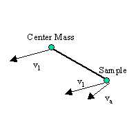
Linear and Angular Velocities

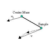
Total Composite Vector

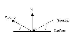
    Using some properties of physics, we know that in a perfect simulation, the angle of incidence is equal to the angle of reflectance.  The angle of incidence is simply the angle between the incoming velocity vector and the normal of the surface.

Reflected Vector

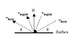
Reflected Linear and Angular Velocities

    First we must normalize the velocity vectors and compute the dot product with the normal to the site.  From this we can compute the reflected ray:

    The reflected ray must then be scaled back to its original magnitude.  By similar methods we can compute the instantaneous force used to repel the rigid body.  Torque can be computed by using the rebound force F:

    In order to make the simulation look realistic, we must introduce scalar quantities that help the physics.  By playing with the scalars we can create the effect of friction that helps with the rotation and torque of the body.  The various scalars can be used to simulate different surface effects, and can be tailored for each voronoi site.  One site may be very slippery, while another can be rough causing a certain 'stickyness' to it so that the body will rotate much faster or dampen the rebound.  The overall effects of using this method for computing the collision forces is very good, and can save time over the impulse based method.

Sampling the Depth Buffer for the Normal

    So far we have talked about computing the normal of a line or point site.  What if we want to use arbitrarily shaped geometry such as bezier curves in our environment?  We already know how to compute the voronoi diagram for such a curve (not discussed here), the problem is how do we compute the normal?  A solution to this is to sample the distance in the depth buffer volumetrically.  By taking samples from the depth buffer that are one pixel away we can look at the local behavior of the bezier curve.  Given these local points we can approximate the normal to the surface.

All Samples on One Side

Sampling on Wrong Side

    Note that this method will work for line and point based voronoi diagrams, although it may not provide the exact answer which can be obtained geometrically from these sites.

An Alternate Way to Compute the Normal

    An alternative method to determining the normal of a voronoi site is to use a more geometric approach to the fixed site.  Instead of having a single line site as previously described, we can create a rectangle out of four voronoi sites.  These sites will have a closed interior which we can special case so that the colors are offset by a certain value, so that if a sample finds these colors it will know that it has penetrated through and correctly compute the normal.
 

Four Voronoi Line Sites

Altered Interiors

    The alternate colors on the interior of the block will allow the solver to detect penetration and correctly compute the normal.  This method can be used for any shape voronoi site.
 

ODE Solver

    Euler's method for computing the motion is a 2^nd order solver that approximates the next value by using the first derivative at the current value.  Given a timestep h that is used to increment the system and a position y at time t_i, Euler's formula states:

    Where y_i' is the first derivative of the position function, velocity in our case.  The value of h directly determines the accuracy of Euler's method.  Keep in mind that h is normally 1/30 or 1/60 depending on how fast (or accurate) you want the simulation to be.  The error in approximation for Euler's method is

    The Runge-Kutta (RK) method of approximation is a 4^th order solver that uses a weighted predictor-corrector strategy to obtain the value at the next timestep.  RK's formula is a bit more complex the Euler's method:

    As you can see RK's error is much smaller by a numerous orders of magnitude.  The difference in calculation between the two systems is noticeable, but for modern day computers should not be a limiting factor in the simulation.  There is also an adaptive RK strategy that will change the value of h appropriately for greater precision.

Performance Hints

The full Voronoi Diagram

The Smaller (More Efficient) Diagram

Future Research

    The methods I have presented for sampling a rigid body are very general methods.  Another possible way to sample the objects is stochaistically.  A random sampling strategy make work very well for some cases.  Exploring this idea will be very useful, especially in 3D rigid body dynamics.

    We've done 2D rigid body dynamics and shown that the collision detection can be done with voronoi diagrams.  What everybody wants is 3D!  My focus this summer will be to explore how to use the voronoi diagram in 3D to perform collison detection in rigid body dynamics.  To perform collision detection we will be using 2D slices of the objects in 3D, should be interesting.  There is a lot of work to be done this summer, check back in the fall for a progress report.

Conclusions