|
|
Fast Penetration Depth Estimation for Elastic Bodies Using Deformed Distance Fields (DDF) |
||
| Susan M. Fisher | sfisher@cs.unc.edu | ||
| Ming C. Lin | lin@cs.unc.edu | ||
PAPER PREPRINT |
|---|
|
Fisher, S. and Lin, M. Fast Penetration Depth Estimation for Elastic Bodies Using Deformed Distance Fields. |
1 COMPUTATION OF AN INTERNAL DISTANCE FIELD |
|---|
|
A distance field is computed by defining the minimum geodesic distance from each point within an object to the object surface. We propose the use of distance fields to estimate penetration depth. Penetration depth is commonly defined as the minimum translational distance required to separate two intersecting objects. When two deformable objects, reaction forces are exerted that result in the deformation of both objects. Penalty-based methods are often used to resolve this contact. Penalty-based methods define a penetration potential energy that measures the degree of intersection between two bodies. One of the more accurate measurements of the amount of intersection is penetration depth. No general and efficient algorithm for computing penetration depth between two deformable objects is known. An approach to compute distance fields for estimating penetration depth between two objects is the Fast Marching Level Set Method. The Fast Marching Method is a technique borrowed from mathematics, and was first introduced by Sethian to track the evolution of interfaces. The equations used are based on the Hamilton-Jacobi equations used in gas dynamics. They are modeled as a conservation law with viscosity. This formulation provides a continuous solution that handle sharp cusps and angles in the object surface. In our algorithm, there are two basic phases: initialization and marching. |
1.1 INITIALIZATION |
|---|
|
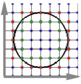
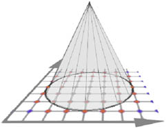
To compute distance values for an arbitrary object requires initializing the location of the surface within a 3D grid. During initialization, a gridpoint may be marked with one of three labels: ALIVE, NARROW_BAND, or FAR_AWAY. An ALIVE point represents a gridpoint who has already been assigned a distance value. A NARROW_BAND point represents a point on the evolving front. A FAR_AWAY point, typically initialized to -infinity, represents a point without an assigned distance value. All gridpoints are first marked FAR_AWAY. The current implementation then makes a pass through each face of the surface, initializing the surrounding gridpoints. To define which gridpoints are neighbors, an axis-aligned bounding box is created around the individual face. Distance values for each gridpoint in the bounding box are then defined. When the initialized value is greater than or equal to zero, the gridpoint lies outside of the object or on the surface. These gridpoints are marked ALIVE. When the distance value is negative, it lies inside the object, and the gridpoint is marked NARROW_BAND. Figure 1 shows an initialized grid for a simple 2D circle; green points represent the NARROW_BAND, red points represent the set of ALIVE points, and blue points are FAR_AWAY.
Figure 1: A 2D example of initialization |
1.2 MARCHING |
|---|
|
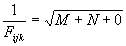
Once the surface has been initialized in the 3D grid, the marching phase of the algorithm may commence. At each step, the gridpoint with the minimum distance value is extracted from the set of NARROW_BAND gridpoints. Upon selection of the minimum valued NARROW_BAND gridpoint, it is marked ALIVE, and any FAR_AWAY neighbors are marked as NARROW_BAND. Each neighbor's distance value is then updated by solving for T in the following equation, selecting the largest possible solution to the quadratic equation:
where
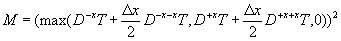
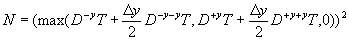
where the finite differences are given by
Similarly, we let
The term Fijk represents the speed of the propagating front. Because we wish to find the distance from each point to the surface, this value is uniform (constant) in this implementation. Figure 2 shows a 2D example of the result of using the Fast Marching Method to compute internal distance fields. The cone represents the linear interpolation of the distance values computed for each gridpoint.
Figure 2: After marching, the cone represents a continuous
|
2 PARTIAL UPDATE OF DDF |
|---|
|
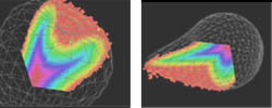
We assume that the collision detection module returns the regions of potential contact. We perform partial updates of the internal distance field by only recomputing the distance values at each grid point within these regions. With such methods as FEM and finite difference methods, this information is easy to obtain. These methods treat objects volumetrically, and therefore they retain information on how far the effects of deformation have propagated throughout the object. Given the bounding box, a second 3D grid is created that overlays the first. The algorithm to compute this partial grid is the same algorithm previously described; the saving in computation time comes from the reduction of the number of grid points being computed. Once the marching completes, we have two datasets that need to be combined while preserving the continuity and differentiability of the solutions.
Figure 3: Partial distance field update of an apple (LEFT)
|
3 QUICKTIME FILES |
|---|
Computation of Distance Field for an Apple
 Shows the computation of a distance field for an apple - Quicktime 9.8MB Shows the computation of a distance field for an apple - Quicktime 9.8MB
|
Computation of Distance Field for a Snake
 Shows the computation of a distance field for a snake - Quicktime 7.2MB Shows the computation of a distance field for a snake - Quicktime 7.2MB
|
Application: Snake Coiling
 (Application of DDF) Shows the automatic coiling motion a snake generated using our FEM simulator - Quicktime 4.6MB (Application of DDF) Shows the automatic coiling motion a snake generated using our FEM simulator - Quicktime 4.6MB
|
Application: Snake Interacting with a Torus
 (Application of DDF) Shows two deformable objects (a snake and a torus) interacting (Application of DDF) Shows two deformable objects (a snake and a torus) interacting
Example 1, Quicktime 5.9MB
|
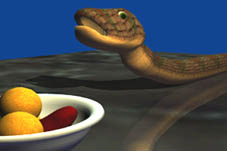
Application: Snake Coiling
 (Application of DDF) A snake swallows an apple, automatically creating bulging motions with our FEM method. Two other renderings are available: transparent (MPEG 2.4 MB) and from the back (MPEG 2.4 MB) (Application of DDF) A snake swallows an apple, automatically creating bulging motions with our FEM method. Two other renderings are available: transparent (MPEG 2.4 MB) and from the back (MPEG 2.4 MB)
|
4 REFERENCES |
|---|
|